pyrestoolbox

A collection of Reservoir Engineering Utilities

This set of functions focuses on those that the author uses often while crafting programming solutions. These are the scripts that are often copy/pasted from previous work - sometimes slightly modified - resulting in a trail of slightly different versions over the years. Some attempt has been made here to make this implementation flexible enough such that it can be relied on as-is going forward.

Modules: gas, oil, brine, nodal (VLP/IPR, VFP tables), simtools (black-oil, PVTW, rel-perm, aquifer and deck tools), dca (decline curves), matbal (material balance), layer, library, recommend and sensitivity. Every module accepts Eclipse METRIC units with metric=True; the full documentation ships inside the package, and pyrestoolbox.docs_dir() returns its location for offline reading.

Includes functions to perform calculations including;

• Decline Curve Analysis with Arps and Duong models - fitting, forecasting, EUR, windowed fitting, secondary phase ratio models, and uptime inference
• Material Balance for gas (P/Z with Cole plot and Havlena-Odeh aquifer support) and oil (Havlena-Odeh with drive indices, parameter regression, and tabulated PVT)
• Inflow Performance Relationships (IPR) for oil and gas wells
• Vertical Lift Performance (VLP) with four multiphase flow correlations (Hagedorn-Brown, Woldesemayat-Ghajar, Gray, Beggs & Brill)
• Nodal analysis operating point determination
• Eclipse VFP table generation (VFPPROD and VFPINJ keywords)
• PVT Calculations for oil
• PVT calculation for gas, including up to 100% inerts for CO2, H2S, N2, H2 and He
• Gas caloric properties (enthalpy, Cp, Cv, Joule-Thomson coefficient) from the BNS tuned Peng Robinson EOS
• Gas hydrate formation prediction with thermodynamic inhibitor calculations
• Return critical parameters for typical components
• Creation of Black Oil Table information (PVDO, PVDG, PVTO, PVTW keywords)
• Creation of layered permeability distribution consistent with a Lorenz heterogeneity factor
• Extract problem cells information from Intersect (IX) print files
• Generation of AQUTAB include file influence functions for use in ECLIPSE
• Creation of Corey, LET and Jerauld relative permeability tables in Eclipse format, with curve fitting support
• Calculation of Methane, CO2 and multicomponent gas saturated brine properties (Soreide-Whitson VLE)
• Multi-salt gas-free brine viscosity: IAPWS-2008 water, an ion-additive salt ratio over any combination of Na, K, Mg, Ca, Sr, Ba, Cl, Br, sulfate and carbonate, and a measured pressure factor
• Method recommendation engine for selecting appropriate correlations based on fluid composition
• Sensitivity analysis with parameter sweeps and tornado charts

All public PVT, flow rate, and simulation table functions support both oilfield (psia, deg F, ft) and Eclipse METRIC (barsa, deg C, m) unit systems via an optional metric=False parameter. See individual module documentation for unit mapping details.

Rust Acceleration (Optional)

pyResToolbox includes optional Rust-compiled extensions that accelerate computationally intensive algorithms. When the compiled extension is present and loadable, these functions run automatically through Rust with no API changes. When the extension is unavailable, all functions fall back silently to the pure Python implementation.

Accelerated functions:

• Nodal VLP segment loops - all 8 VLP method functions (4 methods x gas/oil)
• Gas Z-factor - DAK, Hall-Yarborough, and BNS full-pipeline calculations
• Gas viscosity - LGE and LBC correlations
• Gas pseudopressure - Gauss-Legendre quadrature integration
• Oil density - Standing-Witte-McCain-Hill (iterative and above-Pb)
• Oil FVF - McCain density-based method
• DCA hyperbolic fitting - grid search with RANSAC (fit_decline, fit_decline_cum)
• Material balance - oil matbal regression objective function
• CO2-Brine solubility - Spycher-Pruess iterative RK-EOS solver
• VLE flash - Soreide-Whitson multi-component Peng-Robinson flash

Behavior:

• If the Rust extension is not found on disk, pure Python is used with no warning
• If the extension fails to load (e.g. OS permission restrictions, architecture mismatch), a sentinel file is written to avoid repeated probe attempts on subsequent imports. The sentinel is automatically invalidated when the extension file changes (new build or update)
• All Rust-accelerated paths use try/except wrappers - any Rust-side error falls back to the Python implementation transparently

Environment variables:

• PYRESTOOLBOX_NO_RUST=1 - Force pure Python mode (skip Rust extension entirely)
• PYRESTOOLBOX_RETRY_RUST=1 - Ignore the sentinel file and retry loading the extension

Programmatic status check:

>>> from pyrestoolbox._accelerator import get_status, clear_block
>>> get_status()
{'rust_available': True, 'failure_reason': '', 'forced_python': False, ...}
>>> # If blocked by a sentinel, clear it and restart Python:
>>> clear_block()

Changelist

Upgrade previous installations with

pip install pyrestoolbox --upgrade

Module List

dca	Arps and Duong decline rate and cumulative, EUR estimation, Decline model fitting (time-domain and cumulative, with windowing), Ratio model fitting (GOR/WOR), Forecasting with uptime and secondary phase ratios
matbal	Gas P/Z material balance (OGIP), Cole plot diagnostics, Havlena-Odeh with aquifer influx, Oil Havlena-Odeh material balance (OOIP) with drive indices, Parameter regression with bounds, Tabulated PVT support
gas	Gas Tc & Pc Calculation, Gas Z-Factor Calculation, Gas Viscosity, Gas Viscosity * Z, Gas Compressibility, Gas Formation Volume Factor, Gas Density, Gas Water of Condensation, Convert P/Z to P, Convert Gas Gradient to SG, Delta Pseudopressure, Gas Condensate FWS SG, Gas Flow Rate Radial, Gas Flow Rate Linear, Gas Hydrate Prediction, Gas Caloric Properties (H, Cp, Cv, Joule-Thomson), Non-Darcy and Partial-Penetration Pseudoskins
oil	Oil Density from MW, Oil Critical Properties with Twu, Incremental GOR post Separation, Oil Bubble Point Pressure, Oil GOR at Pb, Oil GOR at P, Oil Compressibility, Oil Density, Oil Formation Volume Factor, Oil Viscosity, Harmonize Pb and Rsb, Estimate soln gas SG from oil, Estimate SG of gas post separator, Calculate weighted average surface gas SG, Oil API to SG, Oil SG to API, Oil Flow Rate Radial, Oil Flow Rate Linear
nodal	Flowing BHP (4 VLP methods), Outflow (VLP) curves, Inflow (IPR) curves, Operating point analysis, Multi-segment deviated/horizontal wells, GasPVT and OilPVT convenience classes
library	Return critical parameters for typical single components
brine	Calculate suite of brine properties with variable methane, Calculate suite of CO2 saturated brine properties, Multicomponent gas-saturated brine (Soreide-Whitson VLE), multi-salt gas-free brine viscosity
layer	Lorenz coefficient from Beta value, Lorenz coefficient from flow fraction, Lorenz coefficient to flow fraction, Lorenz coefficient to permeability array
simtools	Summarize IX convergence errors from PRT file, Create Aquifer Influence Functions, Perform recursive ECL or IX deck zip/check for INCLUDE files, Solve Rachford Rice for user specified feed Zis and Ki's, Create sets of rel perm tables (Corey, LET, Jerauld), Fit relative permeability models to measured data, Generate Eclipse VFPPROD lift curve tables, Generate Eclipse VFPINJ injection curve tables, Create Black Oil tables (PVDO, PVDG, PVTO), Create PVTW water PVT tables
recommend	Recommend Z-factor, critical property, oil PVT, and VLP methods based on fluid composition and well configuration
sensitivity	Parameter sweeps and tornado chart sensitivity analysis

Getting Started

Install the library with pip:

pip install pyrestoolbox

Import library into your project and start using.

A simple example below of estimating oil bubble point pressure.

>>> from pyrestoolbox import oil
>>> oil.oil_pbub(api=43, degf=185, rsb=2350, sg_g=0.72, pbmethod='VALMC')
5199.2406069808885

Fit a decline curve to production data and estimate ultimate recovery.

>>> import numpy as np
>>> from pyrestoolbox import dca
>>> t = np.arange(1, 51, dtype=float)
>>> q = 1000 * np.exp(-0.05 * t)
>>> result = dca.fit_decline(t, q, method='exponential')
>>> result.qi, result.di
(999.9999999999953, 0.049999999999999885)
>>> dca.eur(qi=result.qi, di=result.di, b=0, q_min=10)
19799.999999999953

Estimate gas in place from pressure-production history.

>>> from pyrestoolbox import matbal
>>> r = matbal.gas_matbal(
...     p=[3000, 2700, 2400, 2100, 1800],
...     Gp=[0, 5, 12, 22, 35],
...     degf=200, sg=0.65
... )
>>> r.ogip
87.60264634235122
>>> r.r_squared
0.9734793606102145

A set of Gas-Oil relative permeability curves with the LET method

>>> import matplotlib.pyplot as plt
>>> from pyrestoolbox import simtools
>>> df = simtools.rel_perm_table(rows=25, krtable='SGOF', krfamily='LET', kromax =1, krgmax =1, swc =0.2, sorg =0.15, Lo=2.5, Eo = 1.25, To = 1.75, Lg = 1.2, Eg = 1.5, Tg = 2.0)
>>> plt.plot(df['Sg'], df['Krgo'], c = 'r', label='Gas')
>>> plt.plot(df['Sg'], df['Krog'], c = 'g', label='Oil')
>>> plt.title('SGOF Gas Oil LET Relative Permeability Curves')
>>> plt.xlabel('Sg')
>>> plt.ylabel('Kr')
>>> plt.legend()
>>> plt.grid('both')
>>> plt.plot()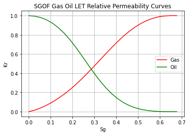

Or a set of Water-Oil relative permeability curves with the Corey method

>>> df = simtools.rel_perm_table(rows=25, krtable='SWOF', kromax =1, krwmax =0.25, swc =0.15, swcr = 0.2, sorw =0.15, no=2.5, nw=1.5)
>>> plt.plot(df['Sw'], df['Krow'], c = 'g', label='Oil')
>>> plt.plot(df['Sw'], df['Krwo'], c = 'b', label='Water')
>>> plt.title('SWOF Water Oil Corey Relative Permeability Curves')
>>> plt.xlabel('Sw')
>>> plt.ylabel('Kr')
>>> plt.legend()
>>> plt.grid('both')
>>> plt.plot()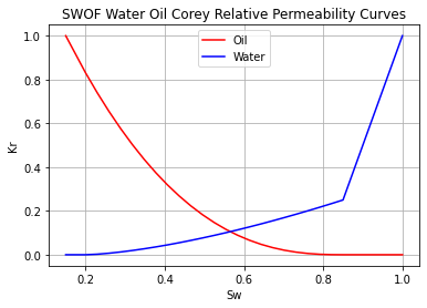

A set of dimensionless pressures for the constant terminal rate Van Everdingin & Hurst aquifer, along with an AQUTAB.INC export for use in ECLIPSE.

>>> ReDs = [1.5, 2, 3, 5, 10, 25, 1000]
>>> tds, pds = simtools.influence_tables(ReDs=ReDs, export=True)
>>>
>>> for p, pd in enumerate(pds):
>>>     plt.plot(tds, pd, label = str(ReDs[p]))
>>>
>>> plt.xscale('log')
>>> plt.yscale('log')
>>> plt.legend(loc='upper left')
>>> plt.grid(which='both')
>>> plt.xlabel('Dimensionless Time (tD)')
>>> plt.ylabel('Dimensionless Pressure Drop (PD)')
>>> plt.title('Constant Terminal Rate Solution')
>>> plt.show()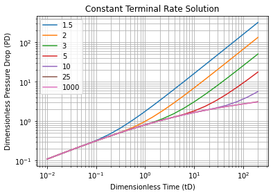

Or creating black oil table information for oil

>>> results = simtools.make_bot_og(pi=4000, api=38, degf=175, sg_g=0.68, pmax=5000, pb=3900, rsb=2300, nrows=50)
>>> df, st_deno, st_deng, res_denw, res_cw, visw, pb, rsb, rsb_frac, usat = results['bot'], results['deno'], results['deng'], results['denw'], results['cw'], results['uw'], results['pb'], results['rsb'], results['rsb_scale'], results['usat']
>>>
>>> print('Stock Tank Oil Density:', st_deno, 'lb/cuft')
>>> print('Stock Tank Gas Density:', st_deng, 'lb/cuft')
>>> print('Reservoir Water Density:', res_denw, 'lb/cuft')
>>> print('Reservoir Water Compressibility:', res_cw, '1/psi')
>>> print('Reservoir Water Viscosity:', visw,'cP')
>>>
>>> fig, ((ax1, ax2), (ax3, ax4)) = plt.subplots(2, 2, figsize=(10,10))
>>> ax1.plot(df['Pressure (psia)'], df['Rs (mscf/stb)'])
>>> ax2.plot(df['Pressure (psia)'], df['Bo (rb/stb)'])
>>> ax3.plot(df['Pressure (psia)'], df['uo (cP)'])
>>> ax4.semilogy(df['Pressure (psia)'], df['Co (1/psi)'])
>>>
>>> fig.suptitle('Black Oil Properties')
>>> ax1.set_title("Rs vs P")
>>> ax1.set_ylabel('Rs (mscf/stb)')
>>> ax1.set_xlabel('Pressure (psia)')
>>> ax1.grid('both')
>>>
>>> ax2.set_title("Bo vs P")
>>> ax2.set_ylabel('Bo (rb/stb)')
>>> ax2.set_xlabel('Pressure (psia)')
>>> ax2.grid('both')
>>>
>>> ax3.set_title("Viso vs P")
>>> ax3.set_xlabel('Pressure (psia)')
>>> ax3.set_ylabel('Viscosity (cP)')
>>> ax3.grid('both')
>>>
>>> ax4.set_title("Co vs P")
>>> ax4.set_ylabel('Co (1/psi)')
>>> ax4.set_xlabel('Pressure (psia)')
>>> ax4.grid('both')
>>>
>>> plt.tight_layout()
>>> plt.show()
Stock Tank Oil Density: 52.06448672566371 lb/cuft
Stock Tank Gas Density: 0.05204687045843109 lb/cuft
Reservoir Water Density: 61.37100825498743 lb/cuft
Reservoir Water Compressibility: 2.930237693350768e-06 1/psi
Reservoir Water Viscosity: 0.36386395924173587 cP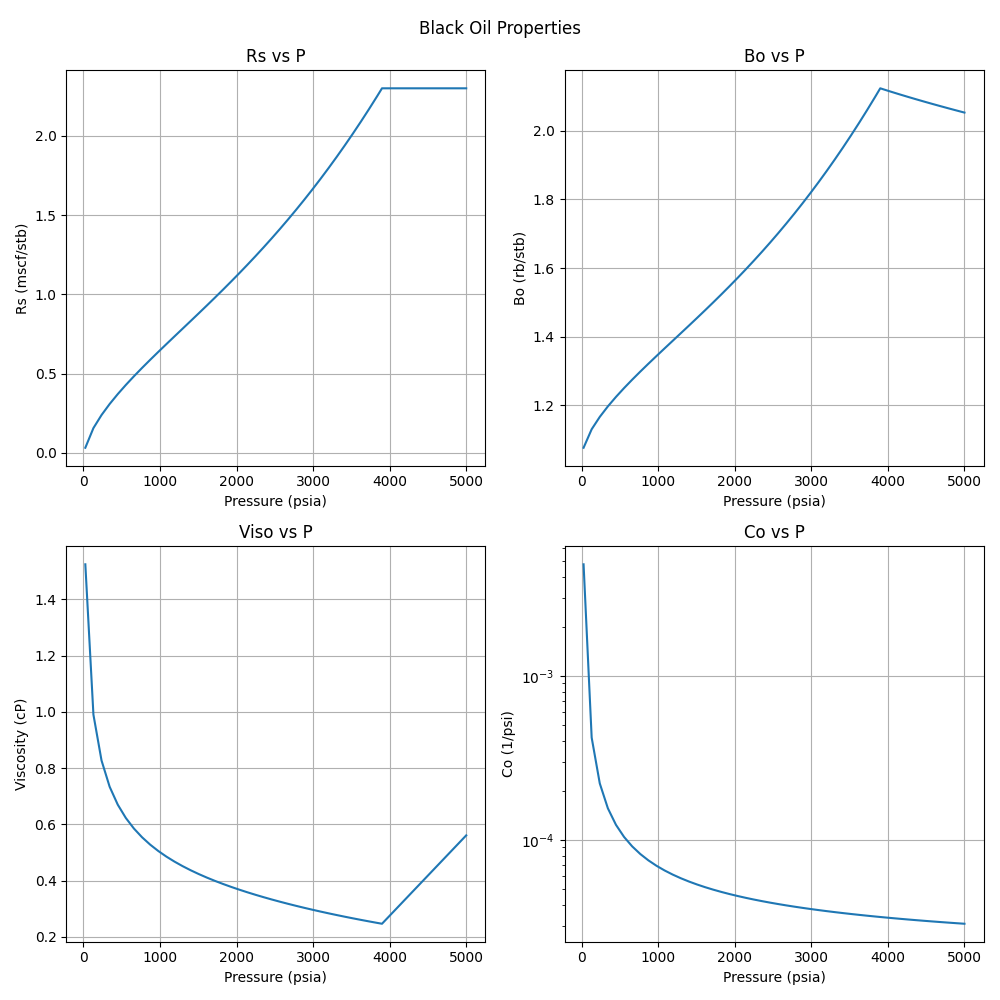

And gas

>>> fig, ((ax1, ax2), (ax3, ax4)) = plt.subplots(2, 2, figsize=(10,10))
>>> ax1.semilogy(df['Pressure (psia)'], df['Bg (rb/mscf'])
>>> ax2.plot(df['Pressure (psia)'], df['ug (cP)'])
>>> ax3.plot(df['Pressure (psia)'], df['Gas Z (v/v)'])
>>> ax4.semilogy(df['Pressure (psia)'], df['Cg (1/psi)'])
>>> ...
>>> plt.show()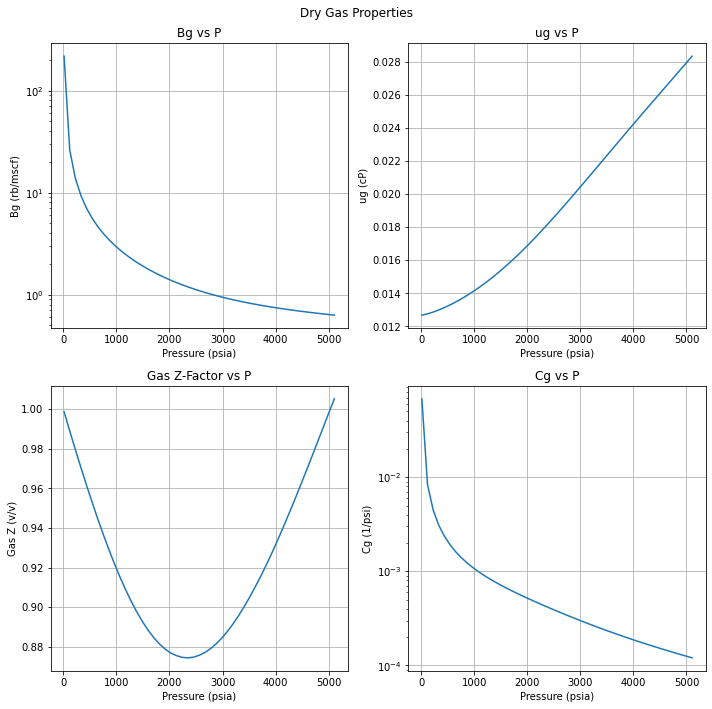

With ability to generate Live Oil PVTO style table data as well

>>> pb = 4500
>>> results = simtools.make_bot_og(pvto=True, pi=4000, api=38, degf=175, sg_g=0.68, pmax=5500, pb=pb, nrows=25, export=True)
>>> df, st_deno, st_deng, res_denw, res_cw, visw, pb, rsb, rsb_frac, usat = results['bot'], results['deno'], results['deng'], results['denw'], results['cw'], results['uw'], results['pb'], results['rsb'], results['rsb_scale'], results['usat']
>>>
>>> if len(usat) == 0:
>>>     usat_flag = False
>>> else:
>>>     usat_flag=True
>>>     usat_p, usat_bo, usat_uo = usat
>>>
>>> try:
>>>     pb_idx = df['Pressure (psia)'].tolist().index(pb)
>>>     bob = df['Bo (rb/stb)'].iloc[pb_idx]
>>>     rsb = df['Rs (mscf/stb)'].iloc[pb_idx]
>>>     uob = df['uo (cP)'].iloc[pb_idx]
>>>     cob = df['Co (1/psi)'].iloc[pb_idx]
>>>     no_pb = False
>>> except:
>>>     print('Pb was > Pmax')
>>>     no_pb = True
>>>
>>> print('Pb (psia):', pb)
>>> print('Bob (rb/stb):', bob)
>>> print('Rsb (mscf/stb):', rsb)
>>> print('Rsb Scaling Required:', rsb_frac)
>>> print('Visob (cP):', uob)
>>> print('Cob (1/psi):', cob,'\n')
>>> print('Stock Tank Oil Density:', st_deno, 'lb/cuft')
>>> print('Stock Tank Gas Density:', st_deng, 'lb/cuft')
>>> print('Reservoir Water Density:', res_denw, 'lb/cuft')
>>> print('Reservoir Water Compressibility:', res_cw, '1/psi')
>>> print('Reservoir Water Viscosity:', visw,'cP')
>>>
>>> fig, ((ax1, ax2), (ax3, ax4)) = plt.subplots(2, 2, figsize=(10,10))
>>> ax1.plot(df['Pressure (psia)'], df['Rs (mscf/stb)'])
>>> ax2.plot(df['Pressure (psia)'], df['Bo (rb/stb)'])
>>> ax3.plot(df['Pressure (psia)'], df['uo (cP)'])
>>> ax4.semilogy(df['Pressure (psia)'], df['Co (1/psi)'])
>>>
>>> ax1.plot([pb], [rsb], 'o', c='r')
>>> ax2.plot([pb], [bob], 'o', c='r')
>>> ax3.plot([pb], [uob], 'o', c='r')
>>> ax4.plot([pb], [cob], 'o', c='r')
>>>
>>> if usat_flag:
>>>     if no_pb == False:
>>>         for i in range(len(usat_bo)):
>>>             ax2.plot(usat_p[i], usat_bo[i], c='k')
>>>             ax3.plot(usat_p[i], usat_uo[i], c='k')
>>>
>>> fig.suptitle('Black Oil Properties')
>>> ..
>>> ..
>>> plt.show()
Pb (psia): 4500
Bob (rb/stb): 1.5372158966466267
Rsb (mscf/stb): 1.137900924344287
Rsb Scaling Required: 1.0362710951888936
Visob (cP): 0.36663121233374113
Cob (1/psi): 2.0042955593519084e-05

Stock Tank Oil Density: 52.06448672566371 lb/cuft
Stock Tank Gas Density: 0.05204687045843109 lb/cuft
Reservoir Water Density: 61.37100825498743 lb/cuft
Reservoir Water Compressibility: 2.930237693350768e-06 1/psi
Reservoir Water Viscosity: 0.36386395924173587 cP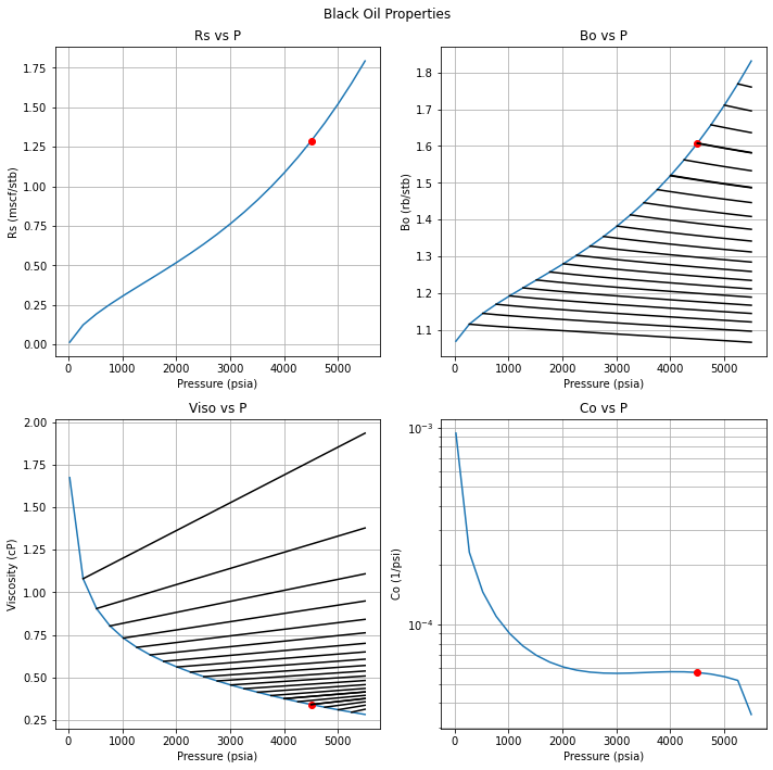

Development

pyrestoolbox is maintained by Mark W. Burgoyne (github.com/mwburgoyne).