Filters

From-scratch implementations of the three classic Bayesian state estimators in Python, presented as runnable Jupyter notebooks with the math derived inline.

Filter	Notebook	Use case
Kalman Filter	src/KalmanFilter.ipynb	Linear systems, Gaussian noise
Extended Kalman Filter	src/ExtendedKalmanFilter.ipynb	Nonlinear systems, Gaussian noise
Error-State EKF (VIO)	src/ErrorStateEKF_VIO.ipynb	State on a manifold (e.g. rotation), IMU + camera fusion
Particle Filter	src/ParticleFilter.ipynb	Nonlinear, non-Gaussian, multi-modal

Install

conda create -n filters python=3.11 -y
conda activate filters
pip install -r requirements.txt
jupyter lab src/

Then open one of the three notebooks listed above.

Kalman Filter

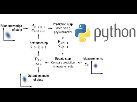
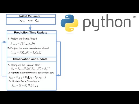
A linear filter — propagates a Gaussian belief through a linear motion model and updates it with linear observations. Optimal under those assumptions.

Predict

$$\hat{\mathbf{x}}_{t \mid t-1} = F , \hat{\mathbf{x}}_{t-1 \mid t-1} + B , \mathbf{u}_t$$

$$P_{t \mid t-1} = F , P_{t-1 \mid t-1} , F^{\top} + Q$$

Update

$$K_t = P_{t \mid t-1} , H^{\top} , \bigl(H , P_{t \mid t-1} , H^{\top} + R\bigr)^{-1}$$

$$\hat{\mathbf{x}}_{t \mid t} = \hat{\mathbf{x}}_{t \mid t-1} + K_t , \bigl(\mathbf{z}_t - H , \hat{\mathbf{x}}_{t \mid t-1}\bigr)$$

$$P_{t \mid t} = (I - K_t , H) , P_{t \mid t-1}$$

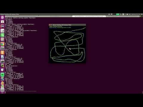
The notebook tracks a moving point in 2D from noisy position measurements and cross-checks against cv2.KalmanFilter. → open notebook

Extended Kalman Filter

Same recursion as the linear Kalman filter, but the linear $F$ and $H$ are replaced with Jacobians of the (nonlinear) motion $g$ and observation $h$ functions evaluated at the current state estimate:

$$J_A = \left.\frac{\partial g}{\partial \mathbf{x}}\right|_{\hat{\mathbf{x}}_{t-1}}, \qquad J_H = \left.\frac{\partial h}{\partial \mathbf{x}}\right|_{\hat{\mathbf{x}}_{t}}$$

$$P_{t \mid t-1} = J_A , P_{t-1 \mid t-1} , J_A^{\top} + Q$$

$$K_t = P_{t \mid t-1} , J_H^{\top} , \bigl(J_H , P_{t \mid t-1} , J_H^{\top} + R\bigr)^{-1}$$

The notebook uses a Constant Turn Rate and Acceleration vehicle model (state: $x, y, \psi, v, \dot\psi, a$) and fuses GPS + IMU + wheel-speed data. The Jacobian is derived symbolically with sympy and shown in the notebook. → open notebook

Error-State Extended Kalman Filter (VIO)

When the state contains a quantity that lives on a manifold — most commonly a rotation in $SO(3)$ — a Gaussian over the full state doesn't make sense, because rotations don't add. The error-state EKF splits the state in two:

• Nominal state $\hat{\mathbf{x}}$ — stored exactly (position, velocity, rotation matrix, IMU biases). Propagated by the full nonlinear IMU integration.
• Error state $\delta\mathbf{x} \in \mathbb{R}^{15}$ — a small additive perturbation around the nominal. Lives in a vector space, so the EKF can track a Gaussian over it.

The Kalman update runs on $\delta\mathbf{x}$ and is then injected back into the nominal state, using $\hat R \leftarrow \hat R \cdot \mathrm{Exp}(\delta\hat\theta)$ for the rotation block so it stays on $SO(3)$:

$$\delta\hat{\mathbf{x}} = K , r, \qquad \hat{\mathbf{x}} \leftarrow \hat{\mathbf{x}} \boxplus \delta\hat{\mathbf{x}}$$

The notebook walks through one complete 15-state ESKF step with full numeric values — IMU propagation, monocular-VO measurement, Kalman update, manifold injection, and Joseph-form covariance update — and verifies every intermediate result against the hand-computed reference. It's also where bias estimation falls out automatically: the gyro/accel biases are corrected through cross-covariances even though the measurement Jacobian has no bias columns. → open notebook

Particle Filter

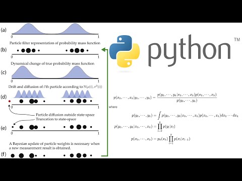
For nonlinear, non-Gaussian, or multi-modal beliefs. Instead of a mean+covariance, the posterior is represented by $N$ weighted samples that are pushed through the motion model, reweighted by the measurement likelihood, and resampled.

Predict — push each particle through the (noisy) motion model:

$$\mathbf{x}_t^{(i)} = f\bigl(\mathbf{x}_{t-1}^{(i)}, \mathbf{u}_t\bigr) + \boldsymbol{\epsilon}^{(i)}, \quad \boldsymbol{\epsilon}^{(i)} \sim \mathcal{N}(0, \Sigma)$$

Weight — for range measurements $z_t^{(\ell)}$ to landmarks $\mathbf{m}^{(\ell)}$:

$$w_t^{(i)} \propto \prod_{\ell} \mathcal{N}\bigl(z_t^{(\ell)} \mid \lVert \mathbf{x}_t^{(i)} - \mathbf{m}^{(\ell)} \rVert, \ R\bigr)$$

Resample — systematic resampling when the effective sample size $N_{\text{eff}} = 1 / \sum_i (w_t^{(i)})^2$ drops below $N/2$.

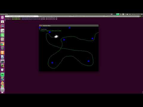
The notebook drives a robot along a synthetic circular trajectory and watches the particle cloud collapse onto the truth as range measurements to six known landmarks accumulate. → open notebook